Keys to Successfully Creating a Birst PPE Inventory Dashboard Set in a Week, Part 4

Part 4: How was it done?

This post will describe, step-by-step, the methods we used to develop this solution in Birst. Parts 1, 2, and 3 of this series laid out the client’s requirements for the project and showed each of the dashboards, described why Infor Birst was the right tool for the job, and laid out the elements that were required for this project’s success.

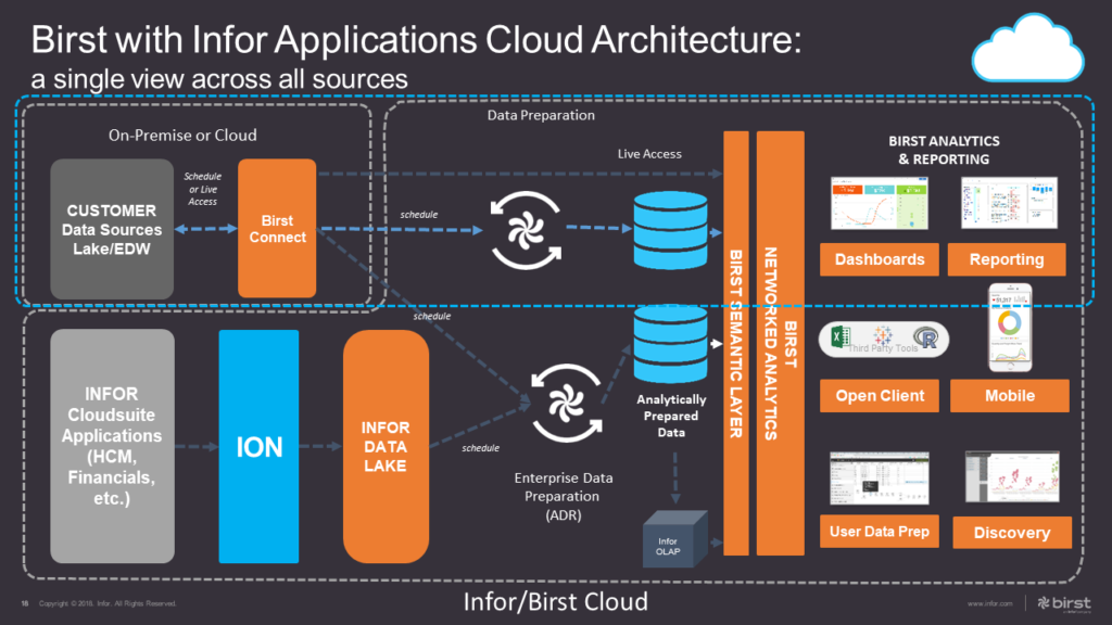
Infor Birst’s Architecture overview:

One of the advantages of the Infor Birst platform is its flexible architecture. As outlined in the image above, Birst can extract data on a schedule from nearly any data source, such as on-prem databases, flat files, Excel files, cloud-based data sources, or even utilize live data sources directly. Extracted data is transformed into analytically prepared data in a multidimensional star schema. The Birst semantic layer makes it easy for different parts of the business to have access to different sets of data, using business logic and names that are relevant to their subject area, and securing access all the way down to the row and column level. Birst’s Networked Analytics lets this data be shared between Birst “spaces” without having to copy data, truly enabling a single source of the truth for reporting. Finally, end-users can consume Birst data in the way that they are most comfortable, most commonly via Birst’s reporting tools (Visualizer and Designer) but also via OCI in applications like Excel and Tableau. Visualizations can be accessed on the web via Birst dashboards directly or embedded in applications like Infor Mingle, Salesforce, or Sharepoint. They can be viewed via the Birst mobile app. Or they can be emailed as attached Excel or PDF files on a schedule or ad hoc.

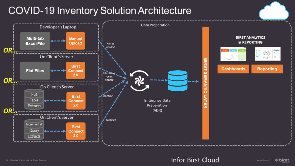
COVID-19 Inventory Solution Architecture:

1. Data sources:
   • While the ultimate solution required database extracts, when this project began they did not have this access sorted out. The database was housed elsewhere and their IT department had to work with the external vendor to provide access. In order to prevent this lack of access from being a blocker to project progress, the project was started using a multi-tab Excel file. The customer provided a small set of sample data with columns that used the business’s common naming for the data content, not the system’s technical names.

Note: Over the course of this short project the data sources were changed from the initial Excel spreadsheet to individual flat files to full data extracts from the source system database to incremental extracts. See the section on Iterative Development below for more on this.

2. Data prep:
   • After uploading the Excel file, the tabs become individual data “sources”, which were then brought into scripts. The scripts were “mapped” to the dimensions and measures of the star schema (see the Relate section below), which are then populated when the data is processed using Birst’s Automatic Data Refinement (ADR).
   • It should be noted that scripts were not strictly necessary at this stage since the sources used the common business terms for the data and the sample data was already in the required format, so no transformations were needed. However, creating scripts NOW made it much easier to update the model later when the data sources were changed to database extracts.
3. User consumption:
   • Most of the end users would be accessing Birst Visualizer reports via the dashboard which was accessible through their Mingle system, although a few were given the ability to log on to Birst directly because they did not have Mingle access. In addition, users were able to sign themselves up for scheduled “notifications”, with the report contents sent to them at their preferred time as Excel email attachments.

Flash End-Of-Life: As you all should know by now, by the end of 2020 the Chrome browser will no longer allow the use of any Flash-based websites, and all major browsers are following their lead (see chromium.org’s Flash roadmap ). Therefore, Infor Birst developers have been hard at work, cranking out improvements to their v7.x HTML5 interface that replaces the old, Flash-based “Classic Admin” interface. Having said that, not all Admin functionality has been added to Birst 7.x yet (see Birst’s Flash end-of-life roadmap). We were able to use the new interface around 95% of the time, but there were a few times when it was necessary to visit the Classic Admin page.

Birst 7.x data modeling workflow: (Connect → Prepare → Relate):

Connect:

• As previously mentioned, the initial data was acquired by uploading a multi-tab spreadsheet by dragging the file from a folder and dropping it on the Upload page within Birst Modeler Connect. The next iteration was to use flat files. They exported data from their database to comma-delimited flat files which they stored on a server within their firewall. Since these files were too large to be manually uploaded to Birst, we decided to create a BirstConnect 2.0 connection for them.
• To set up Birst Connect 2.0 they chose a server that a) was always (or nearly always) available, b) was able to connect to the database server, and c) was able to connect to Birst. You can’t set up a Birst Connect Agent on a server that doesn’t have internet access.
• As per the usual set up routine, they downloaded the Birst Connect 2.0 Local Agent, unzipped it to a folder on their chosen server, and followed the simple directions in the ReadMe file to install the Agent and make it available for use within Birst.
• The flat files that were needed as data sources were placed into the Files folder within the Birst Cloud Agent folder on their server.
• We were then able to create a new Shared Connection in Birst using the new Agent, which gave us access to connect to and extract the data from selected files.
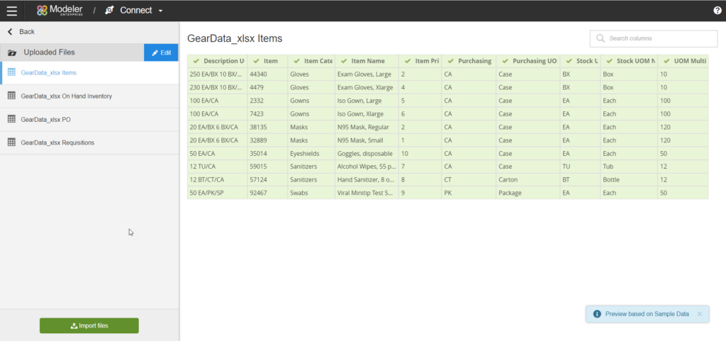
• Once you have set up the connections you need to pull in the raw data by clicking the “Import xxx” button at the bottom of the screen (where “xxx” is the type of data source, like “Files”, or “CRM Data”). See the big green button at the bottom left of Image 3 above.

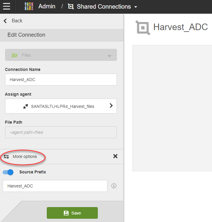
Note: When you include sources from a Shared Connection in a Birst space they will, by default, be prefixed by the connection name. For example, if you have a connection named “FileSource” and you include “File1”, “File2”, and “File3”, the Birst Sources will be named FileSource_File1, FileSource_File2, and FileSource_File3 by default. If you know you will be switching to different sources later, you may wish to turn this prefix off in the Options. See Image 9 below.

Prepare:

• Once you have all your raw sources, the next step is to create any required scripts. Scripts are used for several reasons: to rename columns without losing traceability back to the original column name, to make it easier to change from one raw source to another without impacting the actual model, to transform in the data as needed in ways from simple to complex, and to enable different setups for incremental versus full loads. With Birst 7.x Prepare you can hover your mouse over any source and then click to create a new script from that source.

• Anatomy of a script:
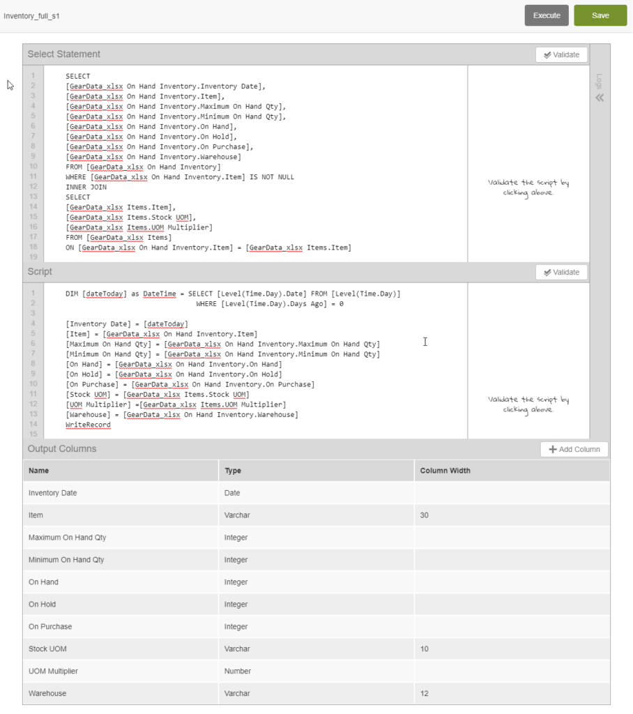
  • Output Columns: Click to edit any script then scroll to the bottom and you will see all of the “Output Columns”. This is the list of columns, with their data types and widths, that will be output as the end result of this script.
  • Select Statement: Scroll back up to the top and you will see the input or “Select Statement” on the top half. This is a Birst Query Language (BQL) query that references raw sources, other scripts, or even the hierarchies and fact tables of the star schema model itself. A BQL query is similar to SQL in that multiple sources can be used, joins can be INNER or OUTER, UNIONS can be used, etc. In this simple example it’s just a simple query referencing the columns of the source that we used to create the script.
  • Script: The middle section is the “Script”. For each row in the “Select Statement”, Birst will execute the code in the “Script” once, moving on to the next row after that. The code can be a simple one-to-one mapping of input column to output column, or it can include sophisticated and complex transformations. In our simple example you will merely see a mapping between the “Output Columns” column name and the input column from the “Select Statement”. An example of a simple transformation might be combining “First Name” and “Last Name” into “Full Name” in the format of “Last Name, First Name”. A more complex transformation would be using an IF THEN ELSE format to determine the value that is output for a particular column based on the input data. As more complexity is needed, more in-depth scripts can be created using WHILE loops, Parent-Child data relationships, variables, mathematical expressions, etc.

Relate:

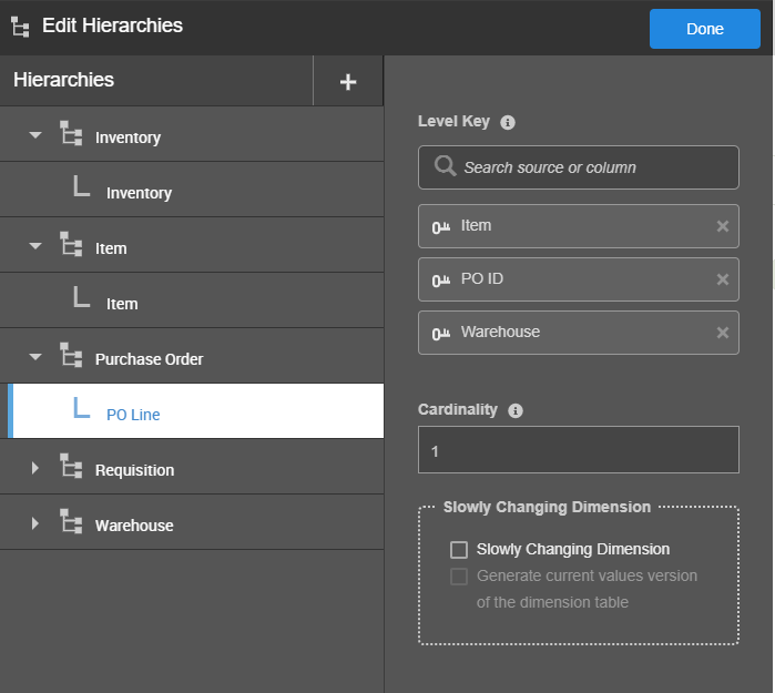
1. First, create each hierarchy and set the level keys (the column or combination of columns that uniquely identifies a row in that hierarchy).
   • Most columns are attributes of a hierarchy. “Company Name” would be an attribute of the “Customer” hierarchy. “Order Status” would be an attribute of the “Purchase Order” hierarchy. “Received Date” would be an attribute of the “Requisition” hierarchy (and it may also be marked as an “Analyse by Date” as mentioned next).
   • In this particular example, we decided that the hierarchies we would have were: Warehouse, Item, Requisition (internal orders of Items to be delivered from their Warehouse to a particular ward or hospital department), Purchase Orders (external orders of Items for the purpose of maintaining stock levels in the Warehouse), and Inventory (the record of what Items in what quantities are in the Warehouse on what Date).
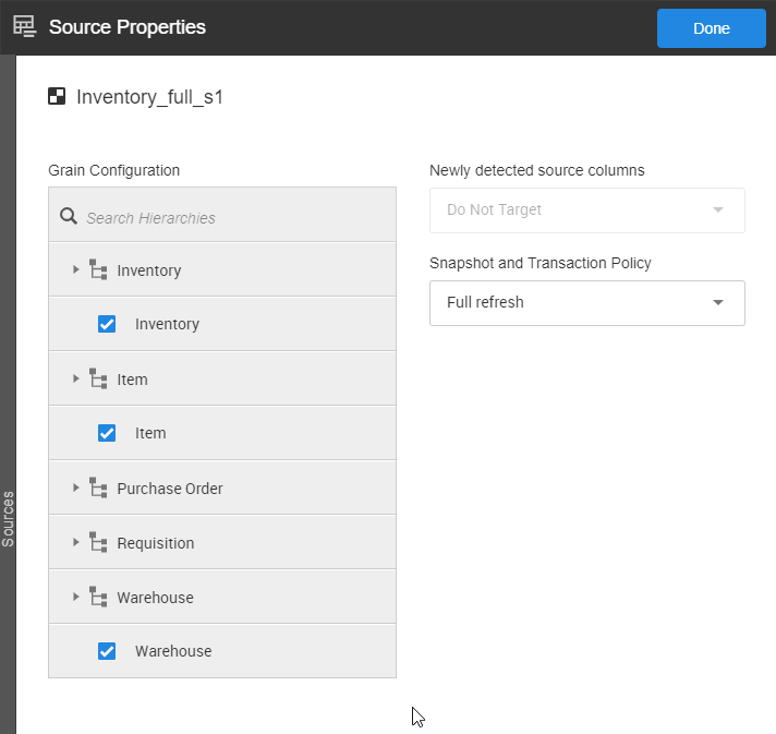
   • Once the columns have been mapped, then the grain and source processing directives need to be set. For example, see Image 6 where the grain of the Inventory_full_s1 script includes the hierarchies Inventory, Item, and Warehouse, and it’s been set to process as a Full Refresh each time.

Tip: Hierarchies/dimensions represent NOUNS and should reflect real-world things, like Customer, Item, Warehouse, Purchase Order, Requisition. They are NOT necessarily a reflection of the raw data sources. They should be a reflection of the way the users understand their business.

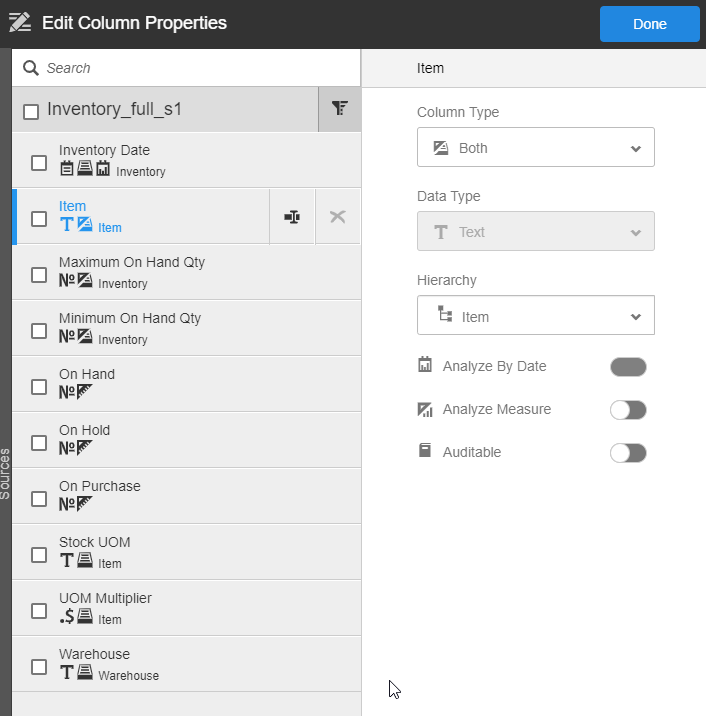
2. Once you’ve created your hierarchies, for each script that should populate the hierarchies, the questions are:
   1. Is this an attribute? If so, of which hierarchy? And/or is this a measure?
   2. Should this date or date/time column be marked as “Analyze by Date”?
3. Measures:
   • A measure is anything you want to count or sum or analyze numerically. Any time you map attributes to more than one hierarchy in a script you will need to have at least one measure in order to connect the data in one hierarchy to the data in another hierarchy. If you don’t have anything in the source that you really want to measure, just choose one of the level key columns.
4. Date columns:
   • Only mark a date column as “Analyse by Date” if you want to be able to use periods of time related to that date as the X axis on a chart (“this measure by month”, “that measure by quarter”) or as a filter (“sales for the year 2020”). If you just need to use it a tabular report but don’t anticipate using it as a chart axis or filter then just make it an attribute, not an Analyze by Date. Use Analyze By Date sparingly because this single check mark impacts the overall model in rather large ways. Going hog wild and checking dozens of unnecessary date columns as Analyze By Date can actually lengthen report rendering time and reduce overall space performance.

Iterative Development:

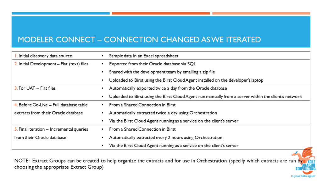
As previously mentioned, the data sources used in this project changed four times in this very brief timeline. As described in the image below, we went from an Excel spreadsheet, to manually-exported flat files, to flat files that were automatically exported twice a day, to full table loads from the Oracle database twice daily, to the final iteration which was incremental table loads from Oracle every two hours throughout the day.

Having to change the data sources over and over manually made some things clear to me that I hadn’t really considered prior to this project.

1. When you use scripts, as recommended above, your script references the source and column names. If you change your sources you can easily change your scripts via find and replace.

Tip: I often copy the top and bottom half of the script into Notepad++ (my favorite text editor), do the find and replace there, and copy them back into Birst. I just find it easier to read in the text editor, although Birst 7.x is admittedly MUCH better than Birst Classic Admin when it comes to working within the script editor directly. Control-Z and tabs work now! Email me if you’re interested in a language file that can be used with Notepad++ to make it easier to work with BQL and Birst log files!

2. If you don’t want to have to change your scripts when you change your sources then you are going to have to use Shared Connections.
3. Ultimately, you will want your new source to have the same name as the source it is replacing, so you want to turn OFF the option to use the connection name as a prefix to the source name.
   • For example, if you have a connection named “SQL_Customer_Data” and you create a query source for that connection and name it “Sales”, then by default the actual name of this source will be “SQL_Customer_Data_Sales”. If you turn OFF the option to use the connection name as a prefix then this source will be named simply “Sales”.

Note: As far as I have been able to tell, the only way to turn this option off is in Shared Connections, so you will want to start using a Shared Connection as soon as possible. In this scenario, we started using a Shared Connection once we got to the 3rd iteration of the data, which was flat files that were automatically output into a folder twice a day. We set them up to be saved into the Files folder within the BirstAgent folder and created a Shared Connection to be used in any of their Birst spaces. We made sure to use the same name for any source in this connection and in the connections we added in later iterations, and we turned off the prefix.

Note: Following the completion of this project, Agile Dragon Consulting anonymized the data, removing all traceability back to the customer or the original source. A separate example space was created so that this information could be shared without compromising data privacy in any way. In the few examples where the requirements or precursor spreadsheets are shown they will be clipped to hide any sensitive information. Otherwise all screenshots and examples in this and future blog posts will be from this example space, not from the actual client’s solution.

Final Thoughts: When I set out to write this series of blog posts I thought it needed to be broken out into four parts. Now that I’ve written the four parts I see so many things I would like to expand on more in future posts. I could easily write 10 parts just on this one project! But, frankly, this post 4 is already too long, so I needed to exert some self-control and just stop writing. There will be more to come in the upcoming weeks (or months) on data modeling in general, and more to come on creating solutions in Birst specifically. If you have any questions or comments, or if you have any suggestions about topics for future blog posts, feel free to email me or comment below.